EMT Toy Model Example

This script can be downloaded as a normal Julia script here.

This example demonstrates an electromagnetic transient (EMT) simulation of a simple two-bus system using PowerDynamics.jl. The system consists of a slack bus connected to a load bus through an RL transmission line, with the load bus having both a dynamic PQ load and a capacitive shunt element.

We compare our simulation results with PowerFactory reference data to validate the EMT modeling approach.

System Description

The test system includes:

• Bus 1: Slack bus (infinite bus with constant voltage)
• Bus 2: Load bus with PQ load and shunt capacitor
• Transmission line: RL model with distributed capacitance
• Disturbance: Load disconnection at t=0.1s

using PowerDynamics
using PowerDynamics.Library
using NetworkDynamics
using ModelingToolkitBase, SciCompDSL
using ModelingToolkitBase: D_nounits as Dt, t_nounits as t
using CSV
using SteadyStateDiffEq
using OrdinaryDiffEqRosenbrock
using OrdinaryDiffEqNonlinearSolve
using DataFrames
using CairoMakie

Per-unit bases

This is a 300 MVA / 110 kV / 50 Hz system. Sbase and the frequency base are global in PowerDynamics: they are set once, before any model is constructed, and every component built afterwards bakes them in. The voltage base is per bus, but this toy system has a single voltage level, so we set the global fallback instead of passing Vbase to each compile_bus call — see the IEEE 9-Bus Example for the per-bus form.

Because the setters are read at construction time, a script that changes them should restore the defaults when it is done, which we do at the very end of this page.

set_Sbase!(300)   # MVA
set_fbase!(50)    # Hz
set_Vbase!(110)   # kV

System Parameters

The component values are given in SI units, so we convert them with the base quantities Zbase and Ybase. Note what the dynamic models below want: not an inductance and a capacitance, but a reactance X = ω₀L and a susceptance B = ω₀C, both in per unit. That is the classical way to parameterize these elements, and it is the convention throughout the library — a pu·s inductance is never an input.

ω0 = get_ωbase()  # Nominal angular frequency [rad/s]

Rline = 1            # Line resistance [Ω]
Lline = (1/100π)     # Line inductance [H]
Cline = (2e-6)       # Line capacitance [F]
Pload = -300         # Load power (negative = consumption) [MW]

# Convert to per-unit reactance/susceptance
Rline_pu = Rline / Zbase(get_Sbase(), get_Vbase())
Xline_pu = ω0*Lline / Zbase(get_Sbase(), get_Vbase())
Bline_pu = ω0*Cline / Ybase(get_Sbase(), get_Vbase())
Pload_pu = Pload / get_Sbase()

Bus Definitions

Slack Bus

The slack bus maintains constant voltage magnitude and angle, representing an infinite bus or strong grid connection.

slackbus = compile_bus(pfSlack(; V=1), vidx=1)

VertexModel :slackbus NoFeedForward() @ Vertex 1
 ├─ 2 inputs:  [busbar₊i_r=-1, busbar₊i_i=0]
 ├─ 0 states:  []
 ├─ 2 outputs: [busbar₊u_r=1, busbar₊u_i=0]
 └─ 6 params:  [busbar₊Vbase=110, systembase₊Sbase=300, systembase₊ωbase=314.16, systembase₊ωframe=1, slack₊V=1, slack₊δ=0]

Dynamic Shunt Capacitor Model

The shunt capacitor is modeled as a dynamic component in the dq-frame. This allows us to observe the three-phase voltages (u_a, u_b, u_c) by transforming from the dq-frame back to abc coordinates.

The capacitor dynamics are given by:

\[\begin{aligned} \frac{B}{\omega_\mathrm{base}}\frac{du_r}{dt} &= -i_r + \omega_\mathrm{frame}\,B\,u_i \\ \frac{B}{\omega_\mathrm{base}}\frac{du_i}{dt} &= -i_i - \omega_\mathrm{frame}\,B\,u_r \end{aligned}\]

This is the classical susceptance form: the capacitance never appears as such, only the susceptance $B = \omega_0 C$ [pu] together with the frequency base $\omega_\mathrm{base}$ [rad/s] that turns it into a physical time constant. The $\omega_\mathrm{frame} B u_i$ and $-\omega_\mathrm{frame} B u_r$ terms are the transport-theorem contribution of the rotating dq-frame; $\omega_\mathrm{frame}$ [pu] is the speed of that frame, pinned to 1. Both come out of the bus' systembase, so the model declares them as shadows with bound_to rather than taking them as its own parameters.

The terminal currents $i_r$ and $i_i$ follow the injector current sign convention: a positive current is defined to flow out of the injector and into the terminal.

@component function DynamicShunt(; name, defaults...)
    @named terminal = Terminal()
    pars = @parameters begin
        B, [description="Shunt susceptance [pu] at ωbase"]
        ωbase, [bound_to = :systembase₊ωbase, description="System frequency base [rad/s]"]
        ωframe, [bound_to = :systembase₊ωframe, description="Global dq frame speed [pu]"]
    end
    vars = @variables begin
        u_r(t), [guess=1, description="Real part of voltage [pu]"]
        u_i(t), [guess=0, description="Imaginary part of voltage [pu]"]
        # Three-phase voltages as observables
        u_a(t), [description="Voltage in a phase [pu]"]
        u_b(t), [description="Voltage in b phase [pu]"]
        u_c(t), [description="Voltage in c phase [pu]"]
    end
    # Transformation matrix from dq to abc coordinates
    Tdqinv(δ) = [cos(δ)       -sin(δ)
                 cos(δ-2pi/3) -sin(δ-2pi/3)
                 cos(δ+2pi/3) -sin(δ+2pi/3)]
    eqs = [
        # Capacitor dynamics in rotating dq-frame
        B/ωbase * Dt(u_r) ~ -terminal.i_r + ωframe*B*u_i,
        B/ωbase * Dt(u_i) ~ -terminal.i_i - ωframe*B*u_r,
        # Terminal connections
        terminal.u_r ~ u_r,
        terminal.u_i ~ u_i,
        # Transform to three-phase voltages; the frame angle advances at ωframe*ωbase
        ([u_a, u_b, u_c] .~ Tdqinv(ωframe*ωbase*t) * [u_r, u_i])...,
    ]
    sys = System(eqs, t, vars, pars; systems=[terminal], name)
    set_mtk_defaults(sys, defaults)
end

Load Bus Components

The load bus combines two components:

1. A PQ load consuming constant active power (injector model from Library)
2. A dynamic shunt capacitor representing line charging

@named load = PQLoad(Pset=Pload_pu, Qset=0)
@named shunt = DynamicShunt(B=Bline_pu)
loadbus = compile_bus(
    MTKBus(load, shunt);
    vidx=2
)

VertexModel :bus PureStateMap() @ Vertex 2
 ├─ 2 inputs:  [busbar₊i_r, busbar₊i_i]
 ├─ 2 states:  [shunt₊u_i≈0, shunt₊u_r≈1]
 ├─ 2 outputs: [busbar₊u_r=1, busbar₊u_i=0]
 └─ 7 params:  [busbar₊Vbase=110, systembase₊Sbase=300, systembase₊ωbase=314.16, systembase₊ωframe=1, load₊Pset=-1, load₊Qset=0, shunt₊B=0.025342]

Transmission Line Model

Dynamic RL Branch

The transmission line is modeled as a dynamic RL branch in the dq-frame. The line current dynamics are given by:

\[\begin{aligned} \frac{X}{\omega_\mathrm{base}}\frac{di_r}{dt} &= (u_{\text{src},r} - u_{\text{dst},r}) - R\,i_r + \omega_\mathrm{frame}\,X\,i_i \\ \frac{X}{\omega_\mathrm{base}}\frac{di_i}{dt} &= (u_{\text{src},i} - u_{\text{dst},i}) - R\,i_i - \omega_\mathrm{frame}\,X\,i_r \end{aligned}\]

where the voltage difference drives the current through the line impedance. As for the shunt, the parameter is the reactance $X = \omega_0 L$ [pu] rather than an inductance, and the frame speed and frequency base come from the line's systembase. Written this way, the steady state is visibly the phasor relation $\Delta u = (R + jX)\,i$ — set the derivative to zero and read off the real and imaginary parts.

Similarly, the line model follows the injector interface at both ends: a positive current is defined as leaving the device and flowing toward the terminals.

@component function DynamicRLBranch(; name, defaults...)
    systems = @named begin
        src = Terminal()
        dst = Terminal()
    end
    pars = @parameters begin
        R, [description="Line resistance [pu]"]
        X, [description="Line reactance [pu] at ωbase"]
        ωbase, [bound_to = :systembase₊ωbase, description="System frequency base [rad/s]"]
        ωframe, [bound_to = :systembase₊ωframe, description="Global dq frame speed [pu]"]
    end
    vars = @variables begin
        i_r(t), [guess=0, description="Current in real part [pu]"]
        i_i(t), [guess=0, description="Current in imaginary part [pu]"]
    end
    eqs = [
        # RL line dynamics in rotating dq-frame
        X/ωbase * Dt(i_r) ~ (src.u_r - dst.u_r) - R*i_r + ωframe*X*i_i,
        X/ωbase * Dt(i_i) ~ (src.u_i - dst.u_i) - R*i_i - ωframe*X*i_r,
        # Terminal current connections (KCL enforcement)
        src.i_r ~ -i_r,  ## Current flows out of source
        src.i_i ~ -i_i,
        dst.i_r ~ i_r,   ## Current flows into destination
        dst.i_i ~ i_i,
    ]
    sys = System(eqs, t, vars, pars; systems, name)
    set_mtk_defaults(sys, defaults)
end

@named branch = DynamicRLBranch(; R=Rline_pu, X=Xline_pu)
line_model = compile_line(
    MTKLine(branch);
    src=1, dst=2
)

EdgeModel :line PureStateMap() @ Edge 1=>2
 ├─ 2/2 inputs:              src=[src₊u_r, src₊u_i] dst=[dst₊u_r, dst₊u_i]
 ├─   2 states:              [branch₊i_i≈0, branch₊i_r≈0]
 ├─ 2/2 outputs:             src=[src₊i_r, src₊i_i] dst=[dst₊i_r, dst₊i_i]
 ├─   7 params:              [src₊Vbase, dst₊Vbase, systembase₊Sbase=300, systembase₊ωbase=314.16, systembase₊ωframe=1, branch₊R=0.024793, branch₊X=0.024793]
 └─   2 params default_from: :src₊Vbase ← src busbar₊Vbase, :dst₊Vbase ← dst busbar₊Vbase

Power Flow Models

PowerDynamics initializes in two steps: solve a static power flow, then bring every dynamic component to the operating point that the power flow prescribes for its terminals — see Powergrid Initialization for the full picture. The part we have to supply is the first step: every component with dynamics needs an algebraic stand-in, attached with set_pfmodel!.

For an EMT model that sounds daunting, but here the stand-ins fall out of the parameterization, because each dynamic element is already described by exactly the quantity its static counterpart wants:

The shunt is the one that is easy to forget: leave it out of the power flow model and the solution is short by the capacitor's reactive injection, so the dynamic model starts next to, but not at, its true operating point.

pf_loadbus = compile_bus(
    MTKBus(PQLoad(; Pset=Pload_pu, Qset=0, name=:load),
           StaticShunt(; G=0, B=Bline_pu, name=:shunt));
    name=:loadbus_pf
)
set_pfmodel!(loadbus, pf_loadbus)

@named branch_pf = PiLine(R=Rline_pu, X=Xline_pu)
set_pfmodel!(line_model, compile_line(MTKLine(branch_pf); name=:line_pf))

Network Assembly and Initialization

With the power flow models in place, we assemble the network and initialize it in a single call. initialize_from_pf solves the power flow, initializes every component against it, and on the way checks that the per-unit bases of all components agree (check_base_consistency).

nw = Network([slackbus, loadbus], line_model)
s0 = initialize_from_pf(nw;verbose=true, subverbose=true)

Initialize VIndex(1) 
 - De-aliased guesses:
   - :busbar₊terminal₊i_i ⇒ :busbar₊i_i ( 0)
   - :busbar₊terminal₊i_r ⇒ :busbar₊i_r ( 0)
 - No free variables! Residual 0.0

Initialize VIndex(2) 
 - De-aliased guesses:
   - :busbar₊terminal₊i_i ⇒ :busbar₊i_i ( 0)
   - :busbar₊terminal₊i_r ⇒ :busbar₊i_r ( 0)
 - Initialization problem is overconstrained (2 vars for 4 equations). Created NonlinearLeastSquaresProblem for:
   - :shunt₊u_i (guess= 0)
   - :shunt₊u_r (guess= 1)
 - Initialization successful with residual 1.3407109778987274e-12
   - :shunt₊u_i => -0.02539
   - :shunt₊u_r =>  0.97451

Initialize EIndex(1) 
 - InitFormulas set:
   - :dst₊Vbase =  110  (via default_from(:dst, :busbar₊Vbase))
   - :src₊Vbase =  110  (via default_from(:src, :busbar₊Vbase))
 - Initialization problem is overconstrained (2 vars for 6 equations). Created NonlinearLeastSquaresProblem for:
   - :branch₊i_i (guess= 0)
   - :branch₊i_r (guess= 0)
 - Initialization successful with residual 1.0292632778694883e-13
   - :branch₊i_i => -0.0020218
   - :branch₊i_r =>  1.0261

Initialized network with residual 2.60023991796482e-11!

The two dynamic states of this system — the capacitor voltage at bus 2 and the line current — now sit at the operating point the power flow prescribes:

(; u_C_r = s0.v[2, :shunt₊u_r], u_C_i = s0.v[2, :shunt₊u_i],
   i_line_r = s0.e[1, :branch₊i_r], i_line_i = s0.e[1, :branch₊i_i])

(u_C_r = 0.9745092559189633, u_C_i = -0.02539048767673276, i_line_r = 1.0261048404483917, i_line_i = -0.002021837486786308)

When there is no static equivalent

This worked because every dynamic model on this page has an obvious algebraic counterpart. That is not always so: an EMT converter model with inner control loops may have nothing you can sensibly write down as a power flow model. The fallback is to solve a neighbouring problem that is easier and use its solution as a guess for the real one.

The detour below shows that for this system. It is a detour: the network simulated further down is nw, initialized above from power flow — nothing here replaces that.

find_fixpoint(nw; alg=DynamicSS(Rodas5P()))

┌ Warning: Verbosity toggle: dt_epsilon
│  At t=4.130168605659392e-5, dt was forced below floating point epsilon 6.776263578034403e-21. Aborting. There is either an error in your model specification or the true solution is unstable (or it cannot be represented in Float64 precision).
└ @ SciMLBase ~/.julia/packages/SciMLBase/jqoB3/src/integrator_interface.jl:1004
┌ Error: NetworkInitError("Could not find fixpoint, solver returned Failure with residual 1.7260147751571128e12 (alg=SteadyStateDiffEq.DynamicSS{Rodas5P{ADTypes.AutoForwardDiff{nothing, Nothing}, Nothing, typeof(OrdinaryDiffEqCore.trivial_limiter!), typeof(OrdinaryDiffEqCore.trivial_limiter!), Nothing}, Float64}(Rodas5P{ADTypes.AutoForwardDiff{nothing, Nothing}, Nothing, typeof(OrdinaryDiffEqCore.trivial_limiter!), typeof(OrdinaryDiffEqCore.trivial_limiter!), Nothing}(nothing, OrdinaryDiffEqCore.trivial_limiter!, OrdinaryDiffEqCore.trivial_limiter!, ADTypes.AutoForwardDiff(), nothing, 20, 0.03), Inf))! For debugging, it is advised to manually construct the steady state problem and try different solvers/arguments:\n\nprob = SteadyStateProblem(nw, uflat(nwstate), pflat(nwpara))\nsol = solve(prob, alg; kwargs...)\nx0 = NWState(nw, sol.u)\n\nFor detail see https://docs.sciml.ai/NonlinearSolve/stable/native/steadystatediffeq/\n")
└ @ Main emt_toymodel.md:323

@component function LessStiffPQLoad(; name, defaults...)
    @named terminal = Terminal()
    pars = @parameters begin
        Pset, [description="Active Power demand [pu]"]
    end
    vars = @variables begin
        i_r(t)=0, [description="Current in real part [pu]"]
        i_i(t)=0, [description="Current in imaginary part [pu]"]
    end
    eqs = [
        # First-order dynamics with fast time constant
        Dt(i_r) ~ 1e3*(-Pset * terminal.u_r/(terminal.u_r^2 + terminal.u_i^2) - i_r),
        Dt(i_i) ~ 1e3*(-Pset * terminal.u_i/(terminal.u_r^2 + terminal.u_i^2) - i_i),
        terminal.i_r ~ i_r,
        terminal.i_i ~ i_i,
    ]
    sys = System(eqs, t, vars, pars; systems=[terminal], name)
    set_mtk_defaults(sys, defaults)
end

@named less_stiff_load = LessStiffPQLoad(Pset=-Pload_pu)
less_stiff_loadbus = compile_bus(
    MTKBus(less_stiff_load, shunt);
    vidx=2
)
less_stiff_nw = Network([slackbus, less_stiff_loadbus], line_model)
less_stiff_s0 = find_fixpoint(less_stiff_nw; alg=DynamicSS(Rodas5P()))

NWState{Vector{Float64}} of Network (2 vertices, 1 edges)
  ├─ VIndex(2, :shunt₊u_i)           => -0.02539048767696604
  ├─ VIndex(2, :shunt₊u_r)           => 0.9745092559815219
  ├─ VIndex(2, :less_stiff_load₊i_i) => 0.026718027183579587
  ├─ VIndex(2, :less_stiff_load₊i_r) => -1.0254613901195122
  ├─ EIndex(1, :branch₊i_i)          => -0.0020218374696187244
  └─ EIndex(1, :branch₊i_r)          => 1.0261048404395847
 p = NWParameter([110.0, 300.0, 314.159, 1.0, 1.0, 0.0, 110.0, 300.0, 314.159, 1.0, 1.0, 0.0253422, 110.0, 110.0, 300.0, 314.159, 1.0, 0.0247934, 0.0247934])
 t = nothing

s0guess = NWState(nw)
# Transfer key state variables from less stiff solution
s0guess[VIndex(2, :shunt₊u_i)] = less_stiff_s0[VIndex(2, :busbar₊u_i)]
s0guess[VIndex(2, :shunt₊u_r)] = less_stiff_s0[VIndex(2, :busbar₊u_r)]
s0guess[EIndex(1, :branch₊i_i)] = less_stiff_s0[EIndex(1, :branch₊i_i)]
s0guess[EIndex(1, :branch₊i_r)] = less_stiff_s0[EIndex(1, :branch₊i_r)]
s0_detour = find_fixpoint(nw, s0guess; alg=DynamicSS(Rodas5P()))

NWState{Vector{Float64}} of Network (2 vertices, 1 edges)
  ├─ VIndex(2, :shunt₊u_i)  => -0.02539048767713425
  ├─ VIndex(2, :shunt₊u_r)  => 0.9745092559190235
  ├─ EIndex(1, :branch₊i_i) => -0.0020218374872394734
  └─ EIndex(1, :branch₊i_r) => 1.0261048404498427
 p = NWParameter([110.0, 300.0, 314.159, 1.0, 1.0, 0.0, 110.0, 300.0, 314.159, 1.0, -1.0, 0.0, 0.0253422, 110.0, 110.0, 300.0, 314.159, 1.0, 0.0247934, 0.0247934])
 t = nothing

maximum(abs, uflat(s0_detour) - uflat(s0))

1.4510614931850796e-12

Disturbance Setup

With the system initialized, we set up a disturbance to observe its transient response. We'll disable the load at t=0.1s to simulate a sudden load disconnection.

disable_load_affect = ComponentAffect([], [:load₊Pset]) do u, p, ctx
    println("Disabling load at time $(ctx.t)")
    p[:load₊Pset] = 0  ## Set load power to zero
end
set_callback!(loadbus, PresetTimeComponentCallback(0.1, disable_load_affect))

Dynamic Simulation

With the system properly initialized and the disturbance configured, we can now run the electromagnetic transient simulation.

prob = ODEProblem(nw, s0, (0.0, 0.15))
sol = solve(prob, Rodas5P());

Disabling load at time 0.1

Results and Validation

We compare our EMT simulation results with PowerFactory reference data to validate the modeling approach. The comparison focuses on the three-phase voltages at bus 2 during the load disconnection transient.

The thick gray lines show the PowerFactory reference, while our PowerDynamics.jl results are overlaid in color. The close agreement validates our EMT modeling approach.

fig = let
    fig = Figure()
    ax = Axis(fig[1,1];
        title="Three-Phase Voltage at Bus 2",
        xlabel="Time [s]",
        ylabel="Voltage [pu]")
    ts = range(0.09, 0.13; length=2000)

    # Load PowerFactory reference data
    df = CSV.read(
        joinpath(pkgdir(PowerDynamics),"docs","examples", "emt_data_minimal.csv.gz"),
        DataFrame
    )
    # Plot PowerFactory results (thick gray lines)
    lines!(ax, df.t, df.u_2_a; label="PowerFactory A", color=:lightgray, linewidth=5)
    lines!(ax, df.t, df.u_2_b; label="PowerFactory B", color=:lightgray, linewidth=5)
    lines!(ax, df.t, df.u_2_c; label="PowerFactory C", color=:lightgray, linewidth=5)

    # Extract and plot our simulation results
    a = sol(ts, idxs=VIndex(2, :shunt₊u_a)).u
    b = sol(ts, idxs=VIndex(2, :shunt₊u_b)).u
    c = sol(ts, idxs=VIndex(2, :shunt₊u_c)).u
    lines!(ax, ts, a, label="PowerDynamics A", color=Cycled(1))
    lines!(ax, ts, b, label="PowerDynamics B", color=Cycled(2))
    lines!(ax, ts, c, label="PowerDynamics C", color=Cycled(3))

    axislegend(ax, position=:rt)
    xlims!(ax, ts[begin], ts[end])
    fig
end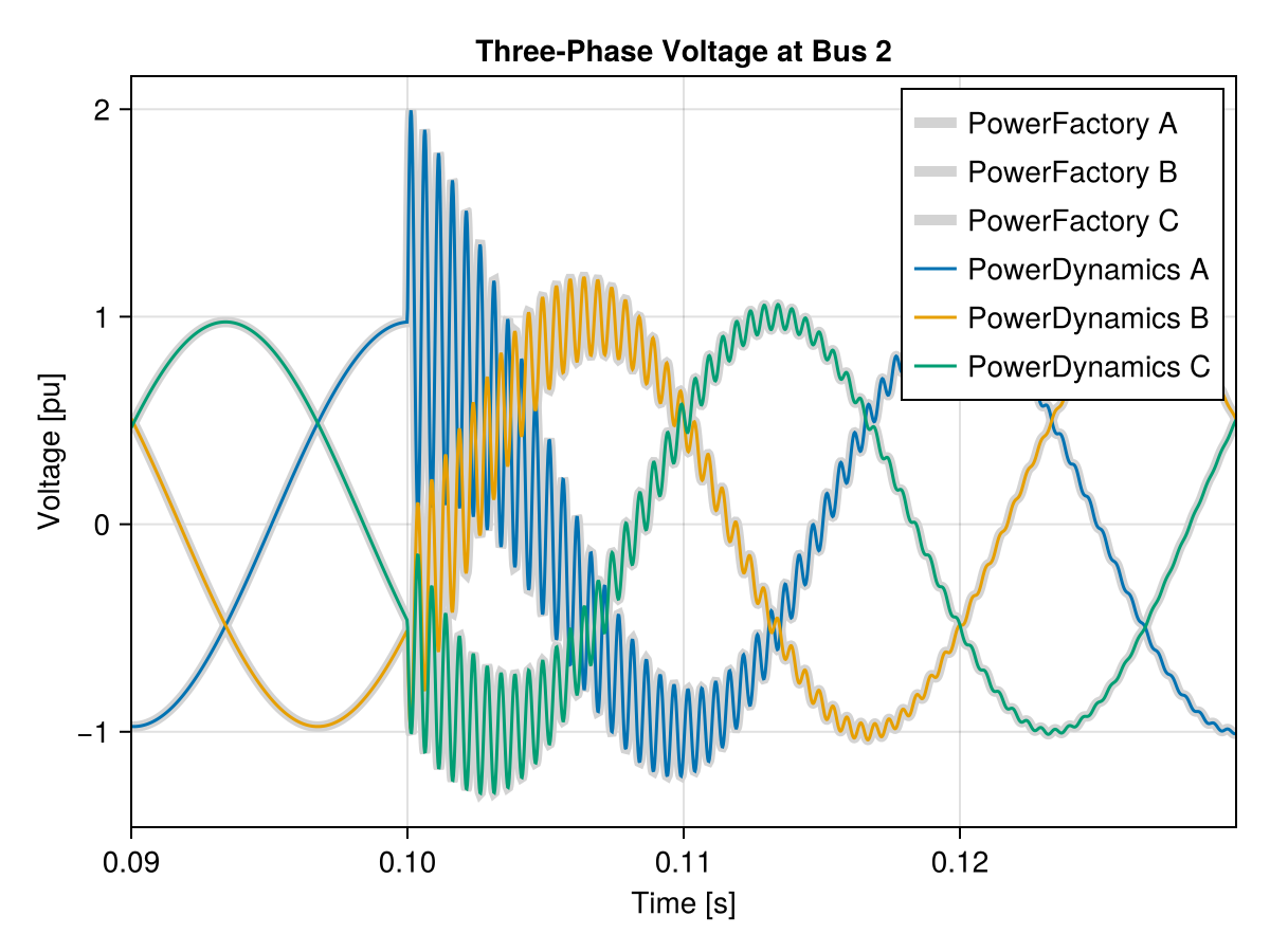

Detailed View of Transient Response

Let's zoom in on the critical period around the load disconnection to better observe the transient behavior and compare with the reference.

xlims!(0.0995, 0.105)
fig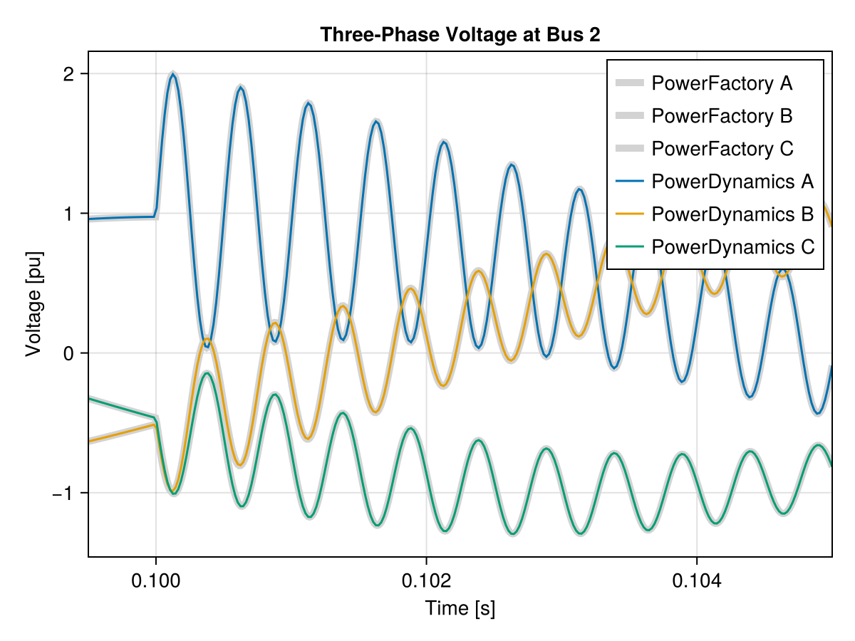

SI observables and restoring the bases

Everything above is in per unit. Because the bases were set before the models were built, every bus and line also carries the SI observables derived from them, so we can read the pre-disturbance voltage of bus 2 in kV rather than converting by hand:

sol(0.099; idxs=VIndex(2, :busbar₊u_kV))

107.23239667893247

Finally, we restore the global bases. Calling the setters without an argument does that, and it keeps this page's 300 MVA / 110 kV from leaking into whatever is constructed next in the same session.

set_Sbase!()
set_fbase!()
set_Vbase!()

This page was generated using Literate.jl.